
The Coronavirus pandemic and climate change are stark examples of the uncertainty that long-term investors face. Their consequences are impossible to predict, forcing investors to think of the future in terms of multiple competing scenarios. Such potential scenarios are not typically intended to capture short-term fluctuations on the market, but rather the longer-term effects of potential market dynamics and developments. Scenario thinking has emerged as a particularly useful tool for pension funds in the process of determining their strategic asset allocation, as a complement to more traditional modelling techniques. The proposed Fragility Score can act as a natural bridge between scenario thinking and traditional Asset and Liability Modelling (ALM).
 The proposed fragility measure captures the sensitivity of an investment portfolio when faced with uncertainty. Traditional optimisation techniques minimise risk, which is defined as deviations from the model. But if the underlying model assumptions do not hold, the investor is faced with uncertainty. A fragile portfolio is sensitive to uncertainty, while a robust portfolio is less so. Having a way to quantify fragility will help long-term investors account for this uncertainty, when choosing between different competing investment portfolios.
This paper has three parts. In the first part we discuss traditional portfolio optimisation and other approaches proposed in the literature for dealing with model misspecification and uncertainty. Second, in a more technical section, the Normalised Fragility Score is derived. Finally, we illustrate how to calculate the fragility measure by using past economic scenarios and discuss how investors can apply this measure in their strategic portfolio construction process when faced with an uncertain future.
PART 1
PORTFOLIO “OPTIMISATION” IN AN UNCERTAIN WORLD CAUSES FRAGILITY
In Markowitz’ (1959) traditional portfolio optimisation, the core assumption is that asset classes follow a multivariate normal distribution and investors have a quadratic utility function. The investor needs to provide estimates of expected returns and the variance-covariance matrix for the available asset classes as well as the risk-aversion parameter “lambda” (l). Based on this, an ‘optimal’ mean-variance portfolio can be calculated. Needless to say, the assumptions underpinning this ‘optimal’ portfolio are quite heroic.
A popular way to estimate the model parameters is to use historical observations. As an improvement, Black and Litterman (1991 and 1992) proposed that investors should calculate the implicit expected return of different assets based on their weight in global markets and the historical variancecovariance matrix. In other words, Black Litterman proposes to use the wisdom of the crowds, rather than historical data, in ‘predicting’ the future. In addition, their approach also allows for investors to provide their own views of how the markets may develop.
The main drawback with both methods is that they magnify small errors in the input, resulting in poor out of sample performance (e.g. Michaud 1989). DeMiguel, Garlappi and Uppal (2009) compare a range of models to a naïve 1/N portfolio and conclude that the naïve portfolio performs consistently better out-of-sample than the optimized ones: ”the gain from optimal diversification is more than offset by estimation errors”. In other words, these optimized portfolios are highly sensitive to the assumptions of future market behavior underpinning the model and are therefore considered “fragile”.
More importantly, the observed dynamics in financial markets are more complex than can be described by a multi-variate normal distribution. The behavior of different actors in markets makes predicting recessions extremely difficult (Borio, Drehmann and Xia, 2019). This is especially the case when the market is faced with an exogenous shock, since the different actors adapt their behaviour to the new situation, which changes the market dynamics in often unpredictable ways. George Soros (1987) called this reflexivity.
As an illustration, in the wake of the Covid-19 crisis, the European Central Bank bought government bonds without adhering to their previously self-imposed capital key. Dutch and German governments abandoned their previously nonnegotiable budget discipline. Institutional investors updated their expectations based on policy changes and expectations of future rescue packages. At this point, we are faced with uncertainty rather than risk (Knight, 1921), since to a large extent it is the mood of consumer and investors that will determine the extent to which the crisis precipitates a negative spiral towards a deflationary depression. The extent of the damage is still not known.
DEALING WITH UNCERTAINTY
Faced with uncertainty, the only thing that is certain is that our assumptions will be wrong. This implies that there is no single mathematical formula for constructing an ‘optimal’ portfolio, but there are some methods that can help improve a portfolio’s resilience, for example, the info-gap theory (Ben-Haim, 2012) where the user can specify how uncertain he/she is of the model and its parameters. In finance literature more has been written about taking uncertainty into account, e.g. Pástor and Stambaugh (2012), who take parameter uncertainty into account when optimizing portfolios. Both these methods focus on adding additional specifications to the model in order to better capture and reflect the uncertainty.
What investors need is a way to reduce the reliance on parametric models. One way to do that is to consider a set of ‘subjective’ scenarios, mapping out how the world could potentially develop. Done carefully, a set of scenarios should cover a broad spectrum of potential outcomes, which is more likely to including the actual outcome, far better than using a framework based on a single parametric model. An alternative to optimizing portfolio returns premised on a set of ‘correct’ assumptions, is to follow a portfolio construction approach targeting robustness of portfolio outcomes under each of the scenarios. Ultimately, this strategy results in building portfolios with satisficing outcomes in case the world develops in the direction of one of the potential scenarios (Lo, 2004).
FACED WITH UNCERTAINTY, THE ONLY THING THAT IS CERTAIN IS THAT OUR ASSUMPTIONS WILL BE WRONG
To provide investors with a framework for applying scenario thinking, we introduce the ‘Fragility Score’. This tool helps investors address the potentially dangerous mismatch between the real world and model assumptions, with the goal of mitigating the fragility of investment outcomes. Our proposed approach can be seen as an augmentation of the traditional Markowitz framework, by introducing an element of uncertainty derived from the forward-looking views underpinning each of the scenarios.
The quality of the Fragility Score is highly dependent on the quality of the scenario set. Some might argue that this will lead to a highly subjective approach. But on the other hand, a narrow and unquestioning belief in one particular parametric model is in itself a very strong subjective view. By reducing our reliance on a single model, we must still acknowledge that future portfolio outcomes might lie beyond the scenario set.
PART II
TRADITIONAL PORTFOLIO “OPTIMISATION”
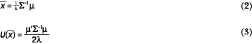
The starting point for deriving the fragility measure is the traditional Markowitz framework for portfolio “optimisation”, which assumes multi-variate normally distributed assets. This approach is frequently applied to everything from tactical deviations from a benchmark portfolio to strategic ALM studies. The popularity of this approach is partly explained by its simplicity. The portfolio weights can be derived analytically from the expected excess returns (m), covariance-matrix (S) and risk-aversion (l) by simply maximising a quadratic utility function:

In its purest form, the optimisation is unconstrained allowing for short positions, cash and leverage. The risk aversion parameter (l) is used to “dial-down” risk, to avoid overly optimised portfolios. A risk aversion between 10 and 20 provides realistic portfolios for the dataset used in the illustration below. The “optimal” portfolio, which maximises the utility for a given risk aversion λ, has a closed form solution, equation (2):
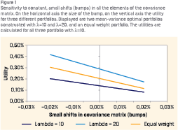 This traditional Markowitz approach is used as the starting point of the fragility measure. Practitioners often introduce a small shift, or a “bump”, to the variance-covariance matrix, through which it is possible to see how sensitive the utility is to small deviations of the parameter estimates or assumptions. Unless the risk-appetite is zero (l ≠ 0), a small shift will cause the expected utility to change. This is illustrated in Figure 1 for three different stylized investment portfolios. Note that this works only for small bumps, such that the covariance matrix remains invertible and economically sensible.
DEFINING THE NORMALISED FRAGILITY SCORE
Inspired by this, we propose a Fragility Score which is based on scenario thinking instead of applying small “bumps”. The investor specifies a set of scenarios, each of which is internally consistent. Instead of measuring the effect of a small “bumps”, the Fragility Score measures the cumulative drop in utility for the portfolio under each scenario (s) belonging to a scenario set (S). The drop in utility can be interpreted as additional ‘pain’ for the investor.
To estimate the fall in utility across all scenarios, an additive operator, see equation (4), is used following Kroll, Levy and Markowitz (1984). This approach makes the fragility-score treat all scenarios with the same weight. The cumulative approach also allows us to calculate the partial-fragility, i.e. the drop in utility for a specific scenario (s ∈ S), which can be used to better identify pockets of fragility
For illustration, a normally distributed multivariate distribution is used in combination with a limited number of scenarios. The base environment is the m, S from which the base case utility U (x) is derived. The scenario set is defined by a discrete number of multivariate distributions. Of course, this methodology can be extended to cover other distributions. It is assumed that each scenario has its own multivariate normal distribution, described by: ms , Ss . The change in utility for a specific scenario is calculated as the difference between the base case utility and the scenario specific utility. The fragility-score is defined as the sum of the utility changes across all scenarios:

The main difference with Kroll et. al. (1984) is that they proposed to first subtract a naïve portfolio’s utility, and then divide the utility by the optimal utility, creating a fractional score. Since the goal is to evaluate utilities across all scenarios, it is not possible to use a fraction. Instead the cumulative ‘drop’ is used which makes it possible to aggregate over any number of scenarios.
It is clear that the quality of the fragility-score is highly dependent on the quality of the scenario set. For more extreme scenarios, the fragility is expected to be higher and vice versa. Following Kroll et. al. (1984) the fragility-score is normalised using the minimum-variance optimal portfolio of the main scenario as the base environment. The normalised fragilityscore is defined as:

The interpretation of the normalised fragility-score is intuitive, as described in Table 1
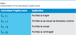 It is worth noting that when the Normalised Fragility Score is negative, the portfolio could be considered ‘antifragile’. Since this measure is based on scenarios, it is only robust against the known unknowns, which is weaker than Taleb (2012) definition of antifragile including the unknown unknowns. For an investor it is attractive to have elements in the portfolio that are antifragile as an insurance against tail risk events, but in most cases, investors target an overall robust portfolio.
PART III
ILLUSTRATING THE NORMALISED FRAGILITY SCORE USING PAST ECONOMIC REGIMES
Historical data is used for illustrating the practical calculation of the Normalised Fragility Score. This allows the variancecovariance matrix to be estimated based on data from different historical economic regimes. In practical applications, the investors do not have the privilege of knowing the future and must therefore provide a scenario set including expected excess return (ms ) and covariance-matrix (Ss ) for each scenario.
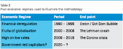 The recent three decades can be divided into three distinct economic regimes as illustrated in Table 2. Typically, an economic regime ends with a crisis. In the volatile aftermath of a crisis, new behaviours are formed and eventually a new regime emerges. This means that a certain investment strategy that worked very well during one specific regime might do poorly in another regime.
The financial deregulation starting in the 80s continued into the 90s, creating a period of high economic growth and booming asset prices. This was followed by a period in which the global economy harvested the fruits of globalisation. In the aftermath of the 2008 financial crisis, Central Banks’ near wholesale shift into low interest rates, while the underlying real economy grew sluggishly. Much more can be said about these three decades, but the key point is that the regimes have been driven by a combination of investor behaviour and policy decisions. This makes the regimes within this time period quite different if we look at the realised returns and traditional measures of risk, such as volatility and correlation between assets. It is worth to note that interest rates have been falling in all regimes.
Looking ahead, it is possible that the Corona pandemic can be one of those events that triggers a transition to a new economic regime. Given the unprecedented governmental and central bank interventions, it is possible that we may we face a regime that can be described as government-led capitalism. This might severely distort the allocation of capital and it may end with a debt crisis in a decade or two. But again, the future is uncharted, so the scenario set must be designed to cover a broad set of possible outcomes.
CALCULATING THE NORMALISED FRAGILITY SCORE
The following example uses historical data to illustrate how an investor can apply the Normalised Fragility Score, when comparing competing portfolios. For the illustration, the competing portfolios consist of cash and three financial assets; real estate, fixed income and equities. The historical returns for these assets in the United States were used as a proxy for historical portfolio returns,1 the returns are expressed in excess of T-bills.2 The dataset comprises of monthly data from 1990 until 2020, i.e. 30 years and 360 observations.
The first step to calculate the Normalised Fragility Score is to establish the base environment. In this example we assume that the Financial deregulation regime covering the period between 1990 and 1999 is the base environment. Realised excess returns are calculated and the variance-covariance matrix is estimated upon data from this period. The unconstrained “optimal” mean- variance portfolio is given by equation (2), using a riskaversion parameter of l = 10. The optimal portfolio weights are; –/–11% in Real Estate (i.e. a short position), 24% in Fixed Income and 67% in Equity. The remaining 20% is held in cash, with a 0% excess return. The realised monthly excess return of this portfolio was 0.72% (annualised excess return of 8.6%), combined with a monthly variance of 0.07% (annualised volatility of 9.3%) resulting in a utility of 0.36%. Due to strong performance of US equity in the 90’s, the Markowitz optimized portfolio is clearly skewed to this asset class.
For the following step in the illustrative example, we have the benefit of hindsight and can compute the normalised Fragility Score by using the two following economic regimes as ‘future’ scenarios. For each scenario the realised excess return is computed, and the variance-covariance matrix is estimated. This provides the ability to calculate the utility of the portfolio for both scenarios.
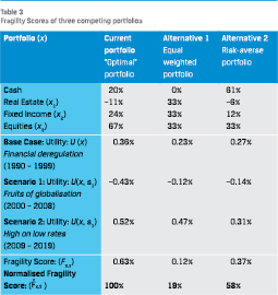 Table 3 shows that for the Fruits of globalisation scenario, covering the period from 2000 to 2008, there is a fall in utility to –0,43%. While for the High on low rates scenario, covering 2009 to 2020, the utility increases to 0,52%. The Fragility Score, i.e. the cumulative drop in utility, was 0,63% in total over the two scenarios and since this is computed for the base case “optimal” portfolio, the Normalised Fragility Score is by definition equal to 100%.
The final step is to compare the base case “optimal” portfolio with the competing portfolios. For this illustration, two alternative investment portfolios are used. The first alternative is an equal-weighted portfolio that is fully invested. The second alternative is a mean-variance optimal portfolio assuming more risk-averse investors (l = 20)3 than the base environment portfolio. In Table 3, the Fragility Score can be found for the base environment, Financial deregulation, as well as the utility for the other two scenarios.
This illustration shows that the “optimal” portfolio under the base environment has, by construction, the highest utility. But in scenario 1, the alternative portfolios have a higher utility than the “optimal” portfolio. The Normalised Fragility Score is 19% respectively, 58% for the two alternative portfolios, which means that they are more robust portfolios than the “optimal” portfolio. This example illustrates how an investor applying scenario thinking can test the relative fragility of competing investment portfolios in order to make better-informed decisions.
LOOKING AHEAD
Investors do not have the benefit of hindsight, nor do they have a crystal ball. In an uncertain world, investors are forced to think in terms of scenarios across economic and market regimes, as to how the future might unfold. The Normalised Fragility Score is an additional tool for the investors toolbox that will help investors choose between different competing investment portfolios. In other words, it augments already used portfolio construction tools like traditional mean variance portfolio optimization and ALM-models.
Looking ahead, there are many events that may impact our society, the economy and financial markets. What are the longterm consequences of the Coronavirus pandemic on the economy? How will climate change impact consumer behaviour and business models? What are the consequences of the aging society? Will addressing inequality within societies and between countries impact the tax on capital versus labour? What will globalisation look like after Pax-Americana? Many of these questions are interconnected by feedback loops which make scenario thinking an attractive approach to be better prepared for dealing with an uncertain future.
INVESTORS DO NOT HAVE THE BENEFIT OF HINDSIGHT, NOR DO THEY HAVE A CRYSTAL BALL
A good example of this is the potential medium to longer-term impact of the Coronavirus pandemic on the local and global economy and subsequent returns on the different asset classes. In order to create an appropriate set of scenarios it is necessary to understand the potential drivers of change, such as; the virus itself, the fragility of the economy and the policy responses, combined existing and advancing issues like climate change and increasing inequality. Understanding those drivers and how they are interconnected allows us to create a set of plausible scenarios and analyse how these may impact both the economy and the financial markets.
To calculate the Normalised Fragility Score, the investor has to choose which of the scenarios should be considered as the base environment. The utility of the current portfolio is then calculated for each of the scenarios. Based on the Normalised Fragility Score for the current investment portfolio, the investor can then analyse the fragility of alternative investment portfolios by comparing their Normalised Fragility Score’s with the current investment portfolio. In other words, the tool provides a practical link between scenario thinking and portfolio construction.
In practice, this tool could prove useful for improving strategic portfolio construction by combining traditional ALM with scenario thinking. In practice, we propose that investors use the Normalised Fragility Score in an iterative process while constructing portfolios. The iterations continue until the portfolio is sufficiently robust and still expected to deliver sufficient investment returns, a process denoted as satisficing (Simon, 1955).
FINAL REMARKS
In this article, we show that a mean-variance “optimal” portfolio is not necessarily optimal from a fragility point of view. The Normalised Fragility Score is one additional tool for the investors toolbox, which can help investors to measure the fragility of their portfolio based on their own scenario set. By definition, the quality of the Fragility Score ultimately depends on the quality of the scenario set that the user provides.
A MEAN-VARIANCE “OPTIMAL” PORTFOLIO IS NOT NECESSARILY OPTIMAL FROM A FRAGILITY POINT OF VIEW
To navigate uncertainty, an investor must have subjective views about how the future might develop. Unfortunately, there are no ‘objective’ views, since narrow and unquestioning belief in the projections of one particular economic model is in itself a very strong ‘subjective’ view. Unless we are willing to wilfully ignore uncertainty, we cannot escape the need for scenario thinking when constructing investment portfolios.
Literature
- Black, F. and R. Litterman, 1991: Asset Allocation Combining Investor Views with Market Equilibrium, Journal of Fixed Income. Vol. 1, No. 2: 718.
- Black, F. and R. Litterman, 1992: Global Portfolio Optimization, Financial Analysts Journal Vol. 48, No. 5: 2843.
- Ben-Haim, Y., 2012 Robust-satisficing and the probability of survival. International Journal of Systems Science. Vol. 45, No 1: 319.
- Borio C., M. Drehmann and D. Xia, 2019. Predicting recessions: financial cycle versus term spread. BIS Working Papers 818. Bank for International Settlements.
- DeMiguel V., L. Garlappi, and R. Uppal, 2009. Optimal versus naïve diversification: How inefficient is the 1/N portfolio strategy? Review of Financial Studies. Vol. 22, No. 5: 191553.
- Knight F., 1921. Risk, uncertainty and profit. University of Illinois at Urbana-Champaign’s Academy for Entrepreneurial Leadership Historical Research Reference in Entrepreneurship.
- Kroll Y., H. Levy and H. Markowitz, 1984. Mean-variance versus direct utility maximization. The Journal of Finance. Vol. 39, No. 1: 4761.
- Lo A., 2004. The adaptive markets hypothesis. The Journal of Portfolio Management. Vol. 30, No. 5: 1529.
- Markowitz H., 1959. Portfolio Selection: Efficient Diversification of Investments. Yale University Press, New Haven.
- Michaud R., 1989. The Markowitz optimization enigma: Is ‘optimized’ optimal? Financial Analysts Journal. Vol. 45, No. 1: 3142.
- Pástor, Ľ. and R. Stambaugh, 2012. Are stocks really less volatile in the long run? The Journal of Finance. Vol 67, No. 2: 431478.
- Simon H., 1955. A behavioral model of rational choice. The quarterly journal of economics. Vol. 69, No. 1: 99118.
- Soros G., 1987. The Alchemy of Finance. John Wiley & Sons Inc., New Jersey.
- Taleb N.N., 2012. Antifragile: how to live in a world we don’t understand. Allen Lane, London.
Notes
- The data used in this article is sourced from Bloomberg. The following indices are used as approximations for the portfolio construction problem: FNERTR Index, LUTLTRUU Index, DJITR Index
- LT12TRUU is used as risk free rate. The monthly returns of the former series are subtracted by the monthly return on the latter.
- Note that we only use a higher risk-aversion for constructing the portfolio, when calculating the utilities, we change it back to l = 10 for a fair comparison.
in VBA Journaal door Rik Klerkx and Stefan Lundbergh