
Over the long-run, risk and return within equity markets are not related. Selecting stocks with a higher risk, does not automatically lead to a higher return (e.g. see a recent discussion on this topic in VBA journaal, by van Vliet (2008) and de Zwart and van Dijk (2009)). This empirical finding contradicts investment theory, which states that higher risk should give a higher expected return. Several explanations for this anomalous finding have been presented in the literature. Blitz and van Vliet (2007) and Baker, Bradley and Wurgler (2011) argue that benchmark driven investors have a relative risk perspective which tends to flatten the risk-return relation. Further Black (1993) argues that leverage restrictions also tend to flatten the risk-return relation.

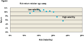
Figure 1 shows the average compounded return of portfolios sorted on historical volatility and beta for the 80-year period from 1931-2009.1 It shows that high-risk stocks are especially unattractive, based both on the return, which is lower, and on risk, which is higher. On the other hand, low-volatility portfolios are especially attractive because they increase the return per unit of risk. The return/risk ratio over the period is 0.68 for the lowest volatility portfolio and steadily decreases to 0.15 for the highestvolatility portfolio.
Based on these empirical results one should avoid the most volatile stocks. For investors with an absolute return focus, for example, investors aiming to maximize the Sharpe ratio, the stocks with the lowest volatility should be selected. Still, it is interesting to investigate how stable these results are over time. Eighty years is a very long time period and much longer than the investment horizon of most investors. If we zoom into the eight different decades comprising the period from 1931-2009, has the relation between risk and return always been negative?
 Never a lost decade
Figure 2 shows the performance of the low/ high volatility decile portfolios for the past eight decades. Interestingly, the low-volatility portfolio had a positive return in each decade. The return varied between 3.4% (2000s) and 19.7% (1980s). By contrast, the high-volatility portfolio had a negative return in three decades (1930s, 1970s, and 2000s). The return of the high-volatility portfolio varied between -9.3% (2000s) and 19.6% (1950s). When we zoom into rolling 10-year windows we find that in 99.4% of all cases the return is positive for the low-volatility compared to 84.3% for the highvolatility portfolio.
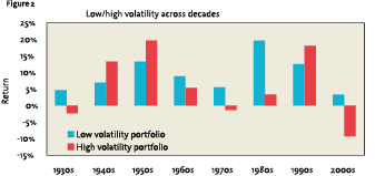 Over the long run, the low-volatility portfolio outperformed the high-volatility portfolio. This was mainly due to avoiding large losses. Still, over several decades high-volatile stocks can also outperform low-volatile stocks. This happened during the 1940s, 1950s and 1990s, when risk and return were positively related. This means that even over a suspended ten-year period, low-volatility stocks can underperform high-volatility stocks. Underperformance in a strong equity market, however, is not very painful from an absolute return perspective. It is worse to have underperformance in a long-term falling market, which is never the case for lowvolatility portfolios. Given the current interest in low-volatility investing, it is important to be aware of the time-varying risk-return relation. Still, the return per unit of risk of low-volatility stocks is superior in each decade, even during the decades (1940s, 1950s and 1990s) when high-volatility stocks outperformed.
 Persistent risk reduction, but no free lunch
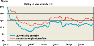
Figure 3 shows the rolling ten-year standard deviation of both the market portfolio and the low-volatility portfolio. During each ten-year period, we observe that the absolute risk of the low-volatility portfolio is lower than that of the market- capitalization weighted index. The volatility of the market varies between 36% and 12%, compared to 25% and 6% for the lowvolatility portfolio. On average, the risk-reduction of the low-volatility portfolio is about 30%, but this varies through time.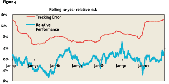
The price investors have to pay to capture this persistent volatility effect is relative risk. One could measure this by calculating the tracking error. From this perspective, low-volatility portfolios are very risky. The average tracking error is about 8% and varies between 4% and 12%. Thus low-volatility investors who compare themselves with market-capitalization weighted indices are faced with very large return differences. Figure 4 shows that over rolling 10-year periods, the annualized return difference can be as large as -4%, which could be a severe career risk for an active fund manager. No one is happy to see 4% annualized underperformance over a ten-year period (-40% in total) and many defensive fund managers lost their jobs in the late 1990s…
Ways to reduce relative risk
 Because of the severe relative risk and thus career risk that comes with low-volatility investing, we also investigate horizon effects. Therefore we also calculate the standard deviation of the return differences over longer-term periods. We find that the tracking error goes down from 8% to 4% when moving from a 10-year to a 20-year investment horizon. In general tracking errors become smaller over longer horizons, but the tracking error goes down sharply because the average returns converge in the long-run. Although the specific investment path is different, the final investment outcome is similar. This additional reduction in tracking error is caused by mean-reversion in relative equity returns.
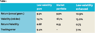
 A way to reduce relative risk in the short term is to add well-known return factors to the low-volatility strategy. A wealth of academic research exists on size, value and momentum effects.2 In this case, we explicitly add value and momentum factors to the low-volatility portfolio.3 The enhanced low-volatility portfolio includes dividend yield and momentum (12-1 month price momentum). The enhanced lowvolatility portfolio is a 70% combination of risk and 30% of dividend yield and momentum.4 Table 1 shows the results, again for the 1931- 2009 period.
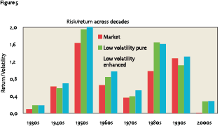
The enhanced portfolio is characterized by a lower tracking error and higher return. The relative risk is reduced from 9.4% to 7.1%. Again we observe that the relative risk goes further down when the horizon is lengthened. A final advantage of the enhanced portfolio is that the return/volatility ratio improves from 0.68 to 0.73. Figure 5 shows that the enhanced portfolio also has an improved risk/return profile across the decades. Especially during the 1940s-1970s period, the return factors help to further improve the low-volatility portfolio. When the rolling 10-year returns are considered then in all (100%) cases the return is positive (versus 99.4% for low volatility). The Sharpe ratio goes up in 79.5% of all 10-year rolling windows, and worsens in 20.5% of the cases. The Sharpe ratio tends to be lower in periods when the return factors underperform the lowvolatility portfolio.
Conclusion
We find that the volatility effect existed during the past 80 years in the US stock market. Risk and return are not positively related, contrary to classic investment theory. In each decade, lowvolatility stocks had a positive absolute return, with lower risk than the market-capitalization weighted index. Still, in some decades, lowvolatility stocks could show underperformance. The main issue with low-volatility investing is tracking error, which could lead to severe underperformance and implies career risk. A focus on long-term performance evaluation and the inclusion of return factors helps to mitigate this relative risk.
References
- Asness, C.S., Moskowitz, T.J., and Pedersen, L.H. (2009), Value and Momentum Everywhere, SSRN working paper no.1363476
- Baker, M.P., Bradley, B., and Wurgler, J.A. (2011), Benchmarks as Limits to Arbitrage: Understanding the Low Volatility Anomaly, Financial Analysts’ Journal, Vol. 67, No. 1, pp. 40-54.
- Banz, R.W. (1981), The Relationship Between Return and Market Value of Common Stocks, Journal of Financial Economics, Vol. 9, No.1, pp. 3-18
- Black, F. (1993), Beta and Return: Announcements of the ‘Death of Beta’ seem Premature, Journal of Portfolio Management, Vol. 20, No. 1, pp. 8-18.
- Blitz, D.C., and van Vliet, P. (2007), The Volatility Effect: Lower Risk Without Lower Return, Journal of Portfolio Management, Vol. 34, No. 1, pp. 102-113.
- Fama, E.F., and French, K.R. (1992), The Cross-Section of Expected Stock Returns, Journal of Finance, Vol. 47, No. 2, pp. 427-465
- Jegadeesh, N., and Titman, S. (1993), Returns to Buying Winners and Selling Losers: Implications for Stock Market Efficiency, Journal of Finance, Vol. 48, No. 1, pp. 65-91
- Vliet, P. van, (2008), Laag risico aandelen prima geschikt voor lange termijn belegger, VBA Journaal, Nr. 3, Najaar 2008, pp. 7-12
- Zwart, G., and van Dijk, R., (2009), Actief omgaan met risico, VBA Journaal, Nr. 3, Najaar 2009, pp. 39-45
Notes
- We create value-weighted decile portfolios for all US stocks. We use 60-months of data to estimate beta and volatility and the decile portfolios are an equal-weighted combination of beta and volatility. We refer to the low-risk portfolios as low-volatility portfolios. We use US data because it is only for this market that such long-term, reliable and clean data are available. Results outside the US have similar or even stronger results (e.g. see Blitz and van Vliet, 2007).
- See Banz (1981) on the size effect, Fama and French (1992) on the value effect and Jegadeesh and Titman (1993) on the momentum effect. For a recent paper on value and momentum investing see Asness, Moskowitz and Pedersen (2009).We obtain data from the data library from Kenneth French.
- We do not explicitly include size in the enhanced portfolio because the size premium has become smaller over time. Some even doubt on the existence of the size premium. Finally, the size effect is implicit in the portfolio since small cap stocks are more likely to be included when stocks are screened on risk, dividend yield and price momentum.
- Three decile portfolios are used to construct the enhanced portfolio: low volatility, high dividend and high price momentum. These are equally mixed with 70% weight for low volatility, 15% weight for dividend and momentum. The Sharpe ratio is not very dependent on the different weightings, but a high weight should be given to low-risk in order to achieve substantial risk reduction. Dividend and momentum decile portfolios are taken from the website of Kenneth French.
in VBA Journaal door Pim van Vliet