
Introduction
Correlation is without doubt the single most important parameter in modern portfolio theory, where it is used to measure the dependence between the returns on different assets or asset classes. The rule is simple: low correlation makes for good diversification and highly correlated assets or asset classes are to be avoided. Fifty years after Markowitz this way of thinking has become so common that nowadays most people use the terms ‘correlation’ and ‘dependence’ interchangeably. When dealing with the normal distributions that modern portfolio theory is based on there is nothing wrong with this. Unfortunately, however, the returns on most assets and asset classes are not exactly normally distributed and tend to exhibit a relatively high probability of a large loss (known formally as ‘negative skewness’) and/or a relatively high probability of extreme outcomes (known as ‘excess kurtosis’). In cases like this correlation is not a good measure of dependence and may actually be seriously misleading. Another problem is that even in cases where correlation is a valid measure of dependence, people do not seem to fully appreciate its exact nature. Although it appears quite surprising at first sight, at least part of the finding that the correlation between hedge fund returns and stock market returns is higher in down than in up markets for example can be attributed purely to technicalities. Even a normal distribution with a constant correlation coefficient will exhibit this sort of behaviour. In this brief note I will discuss these matters in some more detail and provide some examples.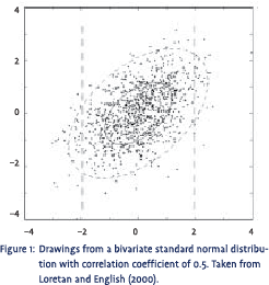
Correlation and non-elliptical distributions
When it comes to correlation and dependence the big question is whether the correlation coefficient is sufficient to describe the complete dependence structure between two variables. Although beyond the scope of this note, it can be shown that this is only the case when the joint (or bivariate) probability distribution of both variables is elliptical. Elliptical simply means that when the joint distribution is viewed from above, the contour lines of the distribution are ellipses. The best-known member of the family of elliptical distributions is of course the normal distribution. From statistics 101 we all know that each and every bivariate normal distribution can be fully described by just two expectations, two variances and one correlation coefficient. Figure 1 shows a plot of a number of drawings from a standard normal bivariate distribution with correlation coefficient 0.5. From the plot we clearly see the elliptical contour shape of the distribution.
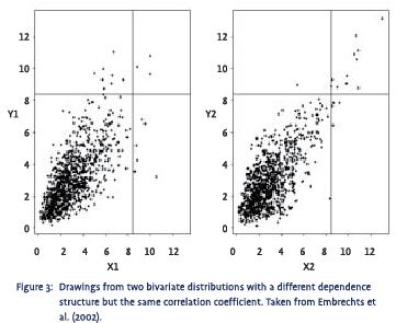
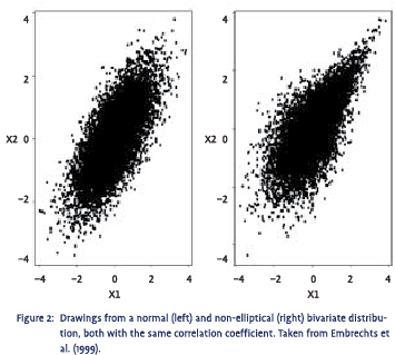 Most real-life distributions exhibit positive or negative skewness and/or some degree of excess kurtosis. Elliptical distributions are therefore nothing more than an ideal type that is rarely encountered in practice. Elliptical distributions, however, are also the easiest distributions to work with mathematically. As a result, the assumption of normality has become the single most important assumption in econometrics, which has left us in the awkward situation where 95% of the econometric tools we have at our disposal assume a distribution that is hardly ever observed in reality.2 As said, if the joint distribution is not elliptical, the correlation coefficient is not a good measure for the dependence structure between the two variables involved. An example is provided in figure 2, which shows plots of a large number of drawings from a normal (on the left) and a non-elliptical (on the right) bivariate distribution. Both plots look very different, implying a completely different dependence structure. The so-called ‘tail dependence’ in the non-elliptical distribution is quite pronounced as it shows a clear tendency to generate extreme values for both variables simultaneously. Surprisingly, however, both these distributions have the same correlation coefficient, which immediately shows how dangerous it can be to rely on just the correlation coefficient to measure dependence. Another example can be found in figure 3. Again, despite the fact that in the distribution on the right there is a much stronger tendency for extreme values to go together, both these distributions have the same correlation coefficient.
In the above context two other points are important as well. First, if two variables are both normally distributed this does not automatically mean that their joint distribution is normal as well. This is only the case if we assume that the joint distribution is elliptical. If not, there are an infinite number of bivariate distributions that fit this description. Second, we all know that because the correlation coefficient equals the normalized covariance, it will always lie between +1 and –1. However, whether it is actually possible for the correlation coefficient to take on these extreme values is another matter. For non-elliptical distributions the actually attainable interval might well be smaller. For some distributions the attainable interval can be very small, say between –0.1 and +0.2 for example. If this was indeed the case, finding a correlation coefficient of 0.2 and concluding that there was only very weak dependence between both variables involved would be a terrible mistake as both variables in question are actually perfectly dependent.
 The above emphasizes how limited the available econometric toolbox still is and how preconditioned we all have become on the assumption of normality. Fortunately, this is changing. More and more econometric research is turning towards non-normal distributions. Also, empirical research no longer aims to show that real-life distributions can be assumed to be normal after all. Partly driven by the fast development of the risk management profession, we seem to be taking things much more the way they really are, i.e. not normally distributed.
Conditional correlations
One way to deal with the problem mentioned above is to calculate what are known as ‘conditional correlations’. This means splitting up the available data sample based on the size or the volatility of one or both of the variables involved and subsequently calculate correlation coefficients for these sub-samples separately. This technique has been used to study the correlation between different assets and asset classes in up and down markets for example. The conclusion is always the same: during major market events correlations go up dramatically. Based on this many investors have come to believe that during times of large moves in financial markets the benefits of (international) diversification are dramatically reduced.
In a recent book, Lhabitant (2002, p. 171) uses the same technique to study the dependence between hedge funds and the stock market. Using data over the period January 1994 to August 2001 he finds that the correlation between most hedge fund indices and US and European equity is much higher in down markets than in up markets. Overall (as measured by the CSFB/Tremont index), the correlation between hedge funds and US equity is 0.18 in up markets but a whopping 0.53 in down markets. The biggest differences between up and down market correlations are observed in convertible arbitrage, emerging markets, and event driven strategies. Similar results can also be found in Schneeweis and Spurgin (2000) and Jaeger (2002, p. 124).
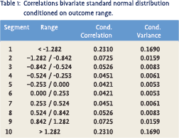 At first sight, findings like the above seem quite worrisome. Fortunately, however, this need not necessarily be the case. It is not difficult to show that conditional correlations should actually display some of the observed behaviour for purely technical reasons. Suppose we had two random variables X and Y with a bivariate standard normal distribution and a correlation coefficient of 0.5, just like the one shown in figure 1. Now suppose we split the range of possible outcomes of X into 10 different segments such that X had exactly 10% chance ending up in either one of these segments. Subsequently, we made a large number of drawings from the bivariate distribution and then calculated the conditional correlation for every segment separately. This would produce the results in table 1. From the table we clearly see that the conditional correlation in segment 1 and 10 is several times higher than in segment 5 or 6, suggesting that large drawings are much more correlated than smaller ones. This is not an empirical observation though, but a purely technical matter as the actual correlation coefficient is fixed.3
It turns out that what is important is the ratio of the conditional variance of X, i.e. the variance within the chosen segment, and the overall variance of X, i.e. the variance calculated over all segments. In our example, the former is given in the last column of table 1 while the latter equals 1 by assumption. The higher the conditional variance relative to the overall variance, the higher the conditional correlation we will find. This means that when we move from the normal distribution to distributions with significant skewness and/or excess kurtosis, the effect may be much stronger. When a distribution is skewed it means that compared to the normal distribution it has a long tail to the left or right. This long tail will raise the conditional variance relative to the overall variance and therefore produce a higher conditional correlation. The same happens with excess kurtosis, i.e. when the distribution in question has ‘fatter’ tails than the normal distribution. When a distribution is sufficiently skewed or leptokurtic this may raise the conditional variance so much that, unlike in the above example, the conditional correlation becomes higher than the unconditional correlation. Since this is a purely technical matter, however, one would be wrong to conclude from this that more extreme movements are more correlated than overall movements.
 Given the above, it is interesting to take another look at Lhabitant’s conditional correlations mentioned before. In a recent paper Brooks and Kat (2001) studied a large number of hedge fund indices, including those studied by Lhabitant. From their study it is clear that the indices that exhibit the biggest difference between up and down market correlation in Lhabitant’s study also happen to be the indices that exhibit the highest levels of negative skewness and excess kurtosis. This strongly suggests that part of Lhabitant’s findings is attributable to technicalities. How much is real is very hard to determine, however, as to do so we would have to know each index’s exact distribution so we could calculate what conditional correlations to expect on purely technical grounds.4
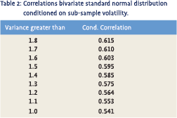
Another interesting example of the dangers of conditional correlations can be found in research that aims to find out whether correlation is higher in more volatile times. This case is quite straightforward because the conditioning is done on the conditional variance itself. We therefore know in advance that the higher we set the threshold of what constitutes high volatility, the more likely we are to find a high conditional correlation. Let’s return to the bivariate standard normal distribution with a fixed correlation of 0.5. Suppose we made a large number of drawings from this distribution, sorted them on whether the absolute value of X was higher or lower than 0.674 and subsequently calculated the conditional correlations of the two resulting sub-samples.
Doing so, we would find a conditional correlation of 0.21 for the small and 0.62 for the high values sample. Many people would be inclined to conclude from this that correlation differs dramatically between volatile and quiet periods. However, this would clearly be incorrect as the correlation is constant by construction. If we sorted the data directly on the variance of X we would get the results displayed in table 2. From the table we clearly see how the conditional correlation rises with the variance threshold, again suggesting that correlation is higher in more volatile markets while by construction it is not.
Conclusion
The above are only simple examples but they make it painfully clear how misleading (conditional) correlation can be. Low (high) correlations do not necessarily imply low (high) dependence. We therefore need other methods to investigate whether for example more extreme movements in financial markets are indeed more highly correlated than overall movements. Given the complexity of real-life distributions, however, such methods are likely to be a lot more complicated than our old friend the correlation coefficient.
Footnotes
- I do not claim any originality with respect to the ideas or even the examples discussed in this note. More details can be found in Boyer et al. (1999), Loretan and English (2000), Embrechts et al. (1999, 2002), or Malevergne and Sornette (2002) and the references therein.
- Note that this is somewhat of an exaggeration as strictly speaking most econometric tools only rely on asymptotic convergence to normality and not on finite sample normality.
- The basic problem here is that the correlation coefficient is dependent on the marginal distributions of the variables in question. Conditioning changes the marginal distributions and thereby changes the correlation coefficient.
- Amin and Kat (2002) find that when forming portfolios of hedge funds, stocks and bonds the negative skewness of the portfolio return distribution increases substantially when the hedge fund allocation is increased. This suggests that a significant part of the observed effect is indeed real.
References
- Amin, G. and H. Kat (2002), Stocks, Bonds and Hedge Funds: Not a Free Lunch!, Working Paper, ISMA Centre, University of Reading.
- Boyer, B., M. Gibson and M. Loretan (1999), Pitfalls in Tests for Changes in Correlations, International Finance Discussion Paper Board of Governors of the Federal Reserve System.
- Brooks, C. and H. Kat (2001), The Statistical Properties of Hedge Fund Index Returns and Their Implications for Investors, forthcoming Journal of Alternative Investments.
- Embrechts, P., A. McNeil and D. Straumann (1999), Correlation: Pitffalls and Alternatives, RISK Magazine, May, pp. 69-71.
- Embrechts, P., A. McNeil and D. Straumann (2002), Correlation and Dependence in Risk Management: Properties and Pitfalls, in M. Dempster (ed.), Risk Management: Value at Risk and Beyond, Cambridge University Press, pp. 176-223.
- Jaeger, L. (2002), Managing Risk in Alternative Investment Strategies, FT Prentice Hall.
- Lhabitant, F. (2002), Hedge Funds: Myths and Limits, Wiley.
- Loretan, M. and W. English (2000), Evaluating Correlation Breakdowns During Periods of Market Volatility, International Finance Discussion Paper Board of Governors of the Federal Reserve System.
- Malevergne, Y. and D. Sornette (2002), Investigating Extreme Dependences: Concepts and Tools, Working Paper Laboratoire de Physique de la Matiere Condensee, University of Nice – Sophia Antipolis.
- Schneeweis, T. and R. Spurgin (2000), Hedge Funds: Portfolio Risk Diversifiers, Return Enhancers or Both, Working Paper CISDM.
in VBA Journaal door Harry M. Kat